Medicare: Building a Data Warehouse from ResDac Files

See also the sibling case study: Medicaid: Building a Data Warehouse from ResDac Files.

This page is the reference documentation for the Medicare data warehouse that Dorieh builds from raw ResDAC files. It walks through the pipeline layer by layer: ingestion of the raw files (Bronze), the cleansed and unified tables and views (Silver), and the QC aggregates (Gold). For a guided path through this page, from the raw ResDAC files to the QC aggregates, start with the tutorial Building the Medicare Claims Pipeline; for a hands-on run against synthetic data, see the example below.

Medallion architecture of the Medicare warehouse 

The Medicare warehouse is organized as a Medallion architecture: data moves through Bronze, Silver, and Gold layers, and each layer is derived only from the layer beneath it.

Bronze: the raw cms.* tables. Every original ResDac file is loaded into its own table, with the data kept as delivered.
Silver: the cleansed and unified layer. It contains the federated views that combine the per-file Bronze tables (medicare.ps and its companion medicare._ps, medicare.mbsf_d, and the admissions view medicare.ip) and the curated tables built from them: medicare.beneficiaries, medicare.enrollments, and medicare.admissions.
Gold: the QC aggregates — the medicare.qc_* materialized views described in Creating QC Tables.

Every ingested (Bronze) table carries two provenance columns: FILE, the name of the original raw file, and RECORD, the line number of the record within that file (see Storing raw data in the Database). These two columns are what make Dorieh’s lineage fine-grained. Column-level lineage records how each output column is computed from input columns, while FILE and RECORD add row-level lineage by anchoring every row to the exact line of the exact source file it came from. Cell-level lineage is the combination of the two: for any single value in a Silver table you can recover both the formula that produced it and the raw record it was derived from.

Processing pipeline 

Medicare Pipeline Steps 

Current pipeline (medicare.cwl) consists of 5 steps, most of them represented as sub-workflows:

initdb: update the Dorieh utilities in the database (see initdb)
Ingest raw data (load_raw_data)
Process beneficiaries and their enrollment in Medicare (enrollments)
Process Admissions (admissions)
Create QC Tables (qc)

Granting SELECT privileges (i.e., read access) to newly created tables is done separately with the standalone grant command line tool; it is not a step of medicare.cwl.

Ingestion of raw data 

Ingestion is incremental: tables already in the database are kept, but any table whose source file is present in the input path is re-created from that file. Every raw record is identified by the tuple (original file name, line number) — the FILE and RECORD provenance columns described above.

Note

If no raw data is given or --input parameters points to a non-existent or empty directory, the pipeline will skip ingestion step and will process the raw data that is already in the database.

Ingestion as a part of the data pipeline is only implemented for data in the format as it comes from ResDac. Metadata for ingestion is taken from FTS files that accompany ResDac deliverables.

Important

For example, in the NSAPH deployment, original ResDAC files in the organization’s possession exist only for the years 2011-2014 and 2016-2018, so in that deployment the pipeline is unable to ingest the data for the other years (1999-2010 and 2015). Readers without access to ResDAC data can run the pipeline against the synthetic dataset described in Example: Medicare Processing Pipeline with Synthetic Data.

See Files for 1999 to 2010 for more information.

See Ingesting Raw Files for processing details

Processing Data in the Database 

During in-database processing all tables, views and materialized views are completely replaced. Old tables are dropped and new ones are created from scratch.

See Combining raw files into unified views for processing details.

Medicare Pipeline References 

See Medicare data ingestion and processing pipeline for the pipeline code

See Medicare data model definition for formal data model definition.

Ingesting Raw Files 

Pipeline

Overview of Ingesting Raw Medicare Files 

There are two types of tables:

Patient summary, aka enrollment, aka denominator
Inpatient admissions

Unfortunately, the structure of medicare files is different for almost every year.

Summary files for some years come in pairs:

mbsf_ab_summary
mbsf_d_cmpnts

For other years we have a single file:

mbsf_abcd_summary

Inpatient admissions files always follow medpar_all_file pattern.

Columns vary from year to year even for similarly named files, new columns are being added and column names are sometimes changed.

A further complication is that for years prior to 2011 (1999-2010) we do not have original files, but preprocessed files with patient summary (called denominators) and admissions. They are in SAS 7BDAT format, however columns are also different for different years. Please refer to Files for 1999 to 2010 section for details.

Storing raw data in the Database 

Given the difference in file structures we create a separate table for every file. However, to make it easier to join these tables we:

Add a column containing original file name to every table
Add generated columns with uniform names for:
- Year
- State
- Bene_Id
- Zip code

In the original files, these data are stored in columns with the following possible names:

Uniform column	Possible source column names
`bene_id`	`bene_id`, `intbid`, `qid`, `bid_5333*`
`state`	`state`, `ssa_state`, `state_code`, `bene_rsdnc_ssa_state_cd`, `state_cd`, `medpar_bene_rsdnc_ssa_state_cd`
`zip`	`zip`, `zipcode`, `bene_zip_cd`, `bene_zip`, `bene_mlg_cntct_zip_cd`, `medpar_bene_mlg_cntct_zip_cd`
`year`	`year`, `enrolyr`, `bene_enrollmt_ref_yr`, `rfrnc_yr`

When a table has no natural primary key (admission tables) we add a record number column. This column has no meaning but makes it possible to trace a record to the original data.

Files for 1999 to 2010 

In the NSAPH deployment, for example, original Medicare ResDAC raw datasets for 1999 to 2010 are not available. Instead, only partially preprocessed files provided by external collaborators exist. These have been stored historically in two separate directories:

denominator/
inpatient/

Each directory contains one file per year. These files use the SAS7BDAT format, which is a binary data format native to SAS analytics software. Each file embeds metadata about its schema (i.e., field names, types, order), but column names and formats still vary from year to year.

To handle this variation:

Each file is individually introspected using the SAS Introspector.
A YAML schema is automatically generated and stored in a central registry.
This schema is then used to create the appropriate database table for ingestion.

For more details on implementation:

See the SAS Introspector for how metadata is extracted.
See the class SAS Data Loader for how these files are ingested into the database.

Because of schema variability:

Special heuristics are used to detect core fields like beneficiary ID ( bene_id), year, zip code, and state code, based on a list of possible alternative names.
Missing expected columns (e.g., year) are sometimes generated using information inferred from directory or file naming.

Each resulting table includes:

A standardized structure with additional generated columns (e.g., record ID, file name).
Uniform field naming conventions to support unioning across years.
Consistent indexing to support later join operations with downstream tables (e.g., beneficiaries and admissions).

Note

Because of the variability and limited provenance of these files, this step is distinct from the ResDAC ingestion workflow and is not based on FTS metadata.

        graph TD;
    A[SAS 7BDAT File] --> B[Inspect schema using SAS Introspector]
    B --> C[Generate YAML metadata]
    C --> D[Update main metadata registry: used for combining tables for all years]
    C --> L[Generate DDL]
    C --> E[Configure SAS Data Loader]
    E --> F[Create SQL table]
    L --> F
    F --> I[Ingest data]
    A --> I
    I --> G[Add synthetic keys and indexes]

Files for Years 2011 and later 

Metadata Extraction 

These files are original files from ResDac. They come in Fixed Width Format (FWF) typically using the .dat extension. Each data file delivered by ResDAC is accompanied by a plain-text metadata file known as a File Transfer Summary (FTS), which describes the structure of the corresponding data file—including:

Column names
Data types (e.g., NUM, CHAR, DATE)
Column widths and formats
Record and file length metadata

These FTS files are designed primarily for human readability and are not machine-friendly. To address this, Dorieh includes a partial FTS parser: the fts2yaml module.

This parser performs the following:

Extracts structured metadata directly from .fts files
Converts it to a standardized YAML-based data model.
- The YaML model describes table and column definitions.
- The YaML model includes types, column widths, descriptions, and indexing hints
Supports both Medicare and Medicaid FTS formats

Once the YAML schema is generated, it is used for:

Generating SQL DDL scripts to create staging tables
Feeding column layout metadata to the FWF reader (FWFReader)
Automatically identifying and indexing key fields such as:
- BENE_ID (Beneficiary ID)
- YEAR
- STATE
- ZIP

Supported File Types 

The parser supports:

Medicare files: identified based on prefixes like mbsf_abcd_XXXX.fts
Medicaid files: using filenames like maxdata_ps_STATE_YEAR.fts

Ingestion process 

Once metadata extraction is complete, raw data ingestion takes place using:

MedicareDataLoader to parse FWF records row-by-row
MedicareLoader to coordinate:
- FTS parsing
- Schema registration
- Loader selection (DAT or CSV)
- Data loading, indexing, and optimization (VACUUM)

The MedicareLoader module orchestrates the end-to-end process, including:

Scanning input directories recursively for *.fts files
Parsing each FTS file to generate a schema
Locating the corresponding *.dat (or *.csv.gz) files
Triggering the appropriate file loader
Writing data to the database

        graph TD;
    A[SAS FTS file] --> B[YAML schema via fts2yaml]
    B --> C[Extract layout for fixed-width reader]
    B --> E[Generate DDL]
    S[SAS DAT FILE] --> D 
    C --> D[Run MedicareLoader calling MedicareDataLoader]
    E --> D
    D --> F[Load data to SQL table]
    F --> G[Apply indexing and VACUUM]

Directory Layout Expectation 

To function correctly with the Dorieh ingestion pipeline, the directory layout for ResDAC raw files must follow this structure:

project_root/
└── medicare/
    └── 2018/
        ├── mbsf_abcd_2018.fts
        ├── mbsf_abcd_2018.dat
        └── medpar_2018.fts

Specifically:

Each year must have its own directory
Table names are inferred from FTS file name and containing year
The FTS filename must match the .dat or .csv.gz data file (just differing in extension)

For a full example of metadata schema outputs, see the Generated Medicare data model.

Combining raw files into unified views 

Pipeline

Eventual database schema 

Once all raw files are ingested into the database they are combined into the unified objects that form the Silver layer of the warehouse:

Patient summary (aka MBSF, aka Beneficiary summary): the medicare.ps view, its companion materialized view medicare._ps, and the medicare.mbsf_d materialized view uniting the split dual-eligibility component files
Inpatient Admissions (aka hospitalizations, aka medpar): the medicare.ip view
The curated tables built from them: medicare.beneficiaries, medicare.enrollments, and medicare.admissions

The figure below visualizes the database schema.

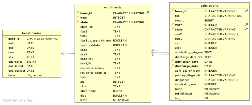
The tables above are defined in Medicare data model definition. This file uses Data Modeling Extensions: Federated Views Across Years.

CWL workflows 

The in-database processing part of the five-step pipeline consists of two sub-workflows:

Creating the beneficiary federated summary and enrollments table
Creating the inpatient admissions table

The QC step is described in Creating QC Tables.

Creating Federated Patient Summary 

The federated patient summary view is created in two steps for purely technical reasons: the second step depends on columns (ssa3, zip) that are cleansed in the first, and splitting the SQL keeps it readable.

This step uses data modeling extensions described in Data Modeling Extensions: Federated Views Across Years.

These steps are part of Medicare Beneficiaries data in-database processing pipeline

First step: Initial in-database data conditioning 

The first step creates a view called medicare.ps.

This step technically combines all cms.mbsf_ab* and cms.mcr_bene_* tables into a single view using CREATE VIEW SQL statement.

It also cleanses and conditions data from the following columns:

year
- If it is a string in original file, it is converted to integer
- If it is two-digit, it is converted to 4 digit
dob: converted to SQL DATE type, from either character or SAS numeric form
dod (date of death): converted to SQL DATE type, from either character or SAS numeric form
age as recorded in the raw data: the beneficiary’s age on January 1 of the given year, if provided in the raw data
sex
race
race_rti Research Triangle Institute (RTI) race code
hmo_indicators Monthly Medicare Advantage (MA) enrollment indicator
hmo_cvg_count Number of months the beneficiary was enrolled
state: added a column with text state id
ssa2: Social Security Administration (SSA) two digit code for state
ssa3: Social Security Administration (SSA) three digit code for county
fips2: added a column with two digit state FIPS code
zip: if original file uses 9-digit zip code, it is split into two separate columns, 5 digit zip and 4-digit zip4. The value is also converted to integer value.
zip4: added, when available - the last four digits of 9-digit zip code

The following CWL tool is responsible to perform it.

Second step: Mapping to county FIPS codes 

At the second step, a materialized view called medicare._ps is created. It adds four computed columns on top of medicare.ps:

fips3: county FIPS code, inferred from the SSA county code (ssa3 column) when it is available, or from the zip code (zip column) when the SSA county code is absent
fips3_is_approximated: flags rows where fips3 had to be inferred from the zip code
fips3_list: all county FIPS codes consistent with the source record
yob: year of birth, calculated from the age variable (year - age)

The reason this has to happen in a separate second step is that both ssa3 and zip are being cleansed in the first step.

The second step is performed by a general loader utility based on the Medicare data model definition.

Creating the mbsf_d dual-eligibility view 

The same sub-workflow (Medicare Beneficiaries data in-database processing pipeline) also creates medicare.mbsf_d, a materialized view that unites the raw cms.mbsf_*d* component tables — the split files that carry the monthly dual-eligibility data for the years in which it is delivered separately. The view keeps the beneficiary id, the year, the number of months of dual coverage (dual_mo) and the array of 12 monthly dual-status indicators (dual_indicators), and it feeds the dual_* column family of the Enrollments table.

Creating Beneficiaries table 

This is also part of Medicare Beneficiaries data in-database processing pipeline

This is also a two steps operation. The first step creates an SQL view and the second step stores the data as a real table.

Essentially it is a medicare.ps view grouped by beneficiary id (bene_id column). This step also takes care of documenting any discrepancies in the data related to:

dob
dod
race
race_rti
sex
orec (the Original Reason for Entitlement Code — see Entitlement reason codes: OREC and CUREC)

If there is any discrepancy for a given bene_id, then:

The earliest DOB is selected as dob
The latest DOD (date of death) is selected as dod
A comma-separated string containing all race codes is used for race
A comma-separated string containing all RTI race codes is used for race_rti
A comma-separated string containing all sex codes is used for sex
The OREC value from the earliest enrollment year is selected as orec (with ties broken by the smallest code, so the result is deterministic)

The following columns are added:

discrepancies: a numeric column counting the alternative values recorded for this beneficiary. It is computed as the number of distinct (dob, race, sex) combinations minus one, plus the number of extra distinct non-null dates of death. A value of 0 means the records are consistent; any value greater than 0 indicates a discrepancy in the raw data for this beneficiary. (Earlier revisions of this page referred to this column as “duplicates”; the physical column name is discrepancies.)
dob_latest: the latest DOB found in the records for this beneficiary. The value of this column is NULL for consistent records
dod_earliest: the earliest DOD found in the records for this beneficiary. The value of this column is NULL for consistent records
orec_latest: the latest OREC value, non-null only when OREC varied across the beneficiary’s records (see Entitlement reason codes: OREC and CUREC)
Beneficiary id HLL hash (bene column), to be used for approximate count distinct queries. See more

The general pattern is defined in Disambiguation rules; the Medicaid page shows an earlier variant of the same approach.

Beneficiary enrollment-span columns 

The beneficiaries table also summarizes each beneficiary’s enrollment history:

first_enrollment_year: the earliest year in which the beneficiary appears in the patient summary data (MIN(year))
last_enrollment_year: the latest such year (MAX(year))
all_enrollment_years: an integer array of all distinct enrollment years, in ascending order
yob: year of birth, the earliest value of year - age computed across the beneficiary’s records; yob_latest is non-null only when the computed year of birth is not the same in all records
number_of_gap_years: the number of years inside the enrollment span for which no enrollment record exists. This column is a worked example of a SQL generated column — it is declared in the data model as
```
GENERATED ALWAYS AS (last_enrollment_year - first_enrollment_year + 1
                     - CARDINALITY(all_enrollment_years)) STORED
```
so PostgreSQL computes and stores the value automatically from the three enrollment-span columns above.

Creating Enrollments table 

This is also part of Medicare Beneficiaries data in-database processing pipeline

Enrollments overview 

Enrollments table contains information about yearly beneficiaries enrollments in different states and tracks changes in eligibility (i.e. beginning of the eligibility and beneficiaries death) and changes in states and addresses.

See also Medicaid Enrollments and Medicaid Eligibility tables. Please note, that since Medicare eligibility is not as volatile as Medicaid eligibility, i.e. it does not usually change month to month, there is no direct analog to Medicaid Eligibility table.

As most of the other tables, Enrollments table is created in two steps. The first step creates an SQL view and the second step stores the data as a real table, adds primary key and builds indices to make queries more efficient.

Enrollments Primary key (unique identifier)

bene_id
year
state

In other words, a record in the table describes a given beneficiary living in a given state during a given year. If beneficiary has moved from one state to another during the year, more than one record for such a beneficiary will be created in the table. This is consistent with Medicaid Enrollments, though, arguably, makes less sense for Medicare.

Enrollments data cleansing 

Beneficiaries can move during a year therefore address columns can have multiple values. These columns are:

fips2: state FIPS code
fips3: county FIPS code
ssa2: SSA state code
ssa3: SSA county code
zip: beneficiary address zip code

The policy for all of these columns is the following:

For the corresponding column in the enrollments table, an arbitrary but deterministic value is selected
For most of these columns an additional companion column is added, containing the list of all encountered values (fips2, which is derivable from the state, has no list column)

Additional columns reflecting data quality and cleansing (state_count, fips3_is_approximated, fips3_valdiated) are also added to the Enrollments table. All of these columns are described in Enrollments columns definitions below.

Enrollments columns definitions 

The following columns are created for Enrollments:

ssa2: SSA state code
ssa3: SSA county code
ssa2_list: list of all SSA state codes
ssa3_list: list of all SSA county codes
state_iso: ISO code of the state, used for mapping
residence_county: one of the “latest” residence counties where the beneficiary was registered, latest in alphabetical order
residence_counties: comma separated list of all “latest” residence counties, where a beneficiary was registered during the year
fips5: 5 digit FIPS code of the residence_county
zip: one of the “latest” zip codes where the beneficiary was registered, latest in numerical order
zips: comma separated list of all “latest” zip codes, where a beneficiary was registered during the year
state_count: number of states, where the beneficiary was enrolled in Medicare during the year. Note, this is also the number of records for this beneficiary and this year in the Enrollments table.
died: a boolean flag indicating that the beneficiary has died during this year while being registered for Medicare in this state.
hmo_indicators: the array of 12 monthly HMO indicators; when the group contains multiple source records, the maximum (by array comparison) of the encountered arrays is kept
hmo_cvg_count: the number of months the beneficiary was enrolled in a Medicare Advantage (MA) plan
hmo: a generated boolean column, true when hmo_cvg_count is greater than zero, i.e. when the beneficiary received benefits through a managed care plan for at least one month of the year; NULL when the count is unknown
buyin_indicators, buyin_cvg_count, buyin (added in a later revision of the data model): the Part B premium buy-in family — an array of the monthly buy-in indicator codes, the number of months during the year when the beneficiary’s premium was paid by the state, and a generated boolean that is true when that count is greater than zero
dual_indicators, dual_cvg_count, dual (added in a later revision of the data model): the dual-eligibility family, taken from the medicare.mbsf_d materialized view (built from the raw mbsf_*d* component files) — an array of the monthly dual-status indicator codes, the number of months of dual coverage during the year (NULL when no mbsf_d data exists for the beneficiary and year), and a generated boolean that is true when that count is greater than zero
curec, curec_latest, consistent_curec: the Current Reason for Entitlement Code and its consistency tracking — see Entitlement reason codes: OREC and CUREC
fips3_is_approximated: A boolean column, indicating whether the value was taken from original record as is or approximated. If true, it means that there was no valid county code in the original ResDac record, hence, the county code was inferred from other data (in most cases, zip code)
fips3_valdiated (sic): A boolean column indicating that the value of county code is consistent with the values of state code and zip code. The physical column name in the database is misspelled exactly as shown here (valdiated, not validated); use this spelling in queries.
Beneficiary id HLL hash (bene column), to be used for approximate count distinct queries. See more

Entitlement reason codes: OREC and CUREC 

Medicare records carry two entitlement reason codes:

OREC (Original Reason for Entitlement Code) records why the beneficiary first became entitled to Medicare. It is set at the time of enrollment and, by definition, never changes for the life of the beneficiary. It is therefore a per-beneficiary invariant and is stored on the beneficiaries table.
CUREC (Current Reason for Entitlement Code) records the current reason for entitlement and can legitimately change from year to year. It is therefore a year-varying attribute and is stored on the enrollments table.

This split is a rule of the data model, not just tidiness. The QC view qc_enrl_bene is defined as enrollments NATURAL JOIN beneficiaries, and in a natural join every column present in both tables becomes part of the implicit join key. If a column such as orec were kept on both tables, every row where the two values disagree would silently drop out of the join — no error, no warning, just missing rows and understated counts downstream. To keep the natural join keyed only on the true relationship (the beneficiary id), per-person invariants must live only on beneficiaries and year-varying attributes only on enrollments.

How the two codes are computed:

beneficiaries.orec takes its canonical value from the earliest enrollment year, with ties broken by the smallest code so that the result is deterministic: (array_agg(orec ORDER BY year, orec))[1]. If the raw data nevertheless shows OREC changing over the years, beneficiaries.orec_latest is non-null (holding the latest value), and the consistent_orec flag in qc_enrl_bene reports the discrepancy: MISSING when OREC is absent, AMBIGUOUS when it varied, and CONSISTENT otherwise. This is the same earliest-value-canonical, latest-value-in-a-secondary-column disambiguation pattern used for the date of birth (dob / dob_latest / consistent_dob).
enrollments.curec is aggregated as MAX(curec) within each (bene_id, year, state) group. This is a defensive de-duplication: in the synthetic dataset every such group is a single row, but real Medicare data can contain duplicate source rows (for example, from overlapping or reissued MBSF files) that disagree on CUREC. When that happens, curec_latest is non-null and the consistent_curec flag is AMBIGUOUS; otherwise it is CONSISTENT (or MISSING when CUREC is absent). Because CUREC consistency is a property of a single enrollment year — not of the beneficiary across years — consistent_curec is a generated, stored column on the enrollments table itself, deliberately not one of the beneficiary-grain flags computed in qc_enrl_bene. It still reaches the qc_enrollments aggregates through the join.

Design note — evolved after the book

Earlier revisions of the data model kept a per-year orec column on enrollments, making it an implicit key of the natural join described above. The current model removes it and surfaces disagreements through orec_latest / consistent_orec, with curec_latest / consistent_curec doing the same for CUREC.

Creating Federated Admissions view 

This step is part of Process Medicare inpatient admissions data inside the database

This step technically combines all cms.medpar* and cms.mcr_ip_* tables into a single view using CREATE VIEW SQL statement. The result is the medicare.ip view.

It also cleanses and conditions data from the following columns:

year
- If it is a string in original file, it is converted to integer
- If it is two-digit, it is converted to 4 digit
state: added a column with text state id
fips2: added a column with two digit state FIPS code
zip: if original file uses 9-digit zip code, it is split into two separate columns, 5 digit zip and 4-digit zip4. The value is also converted to integer value.
zip4: added, when available - the last four digits of 9-digit zip code
admission_date: converted to SQL DATE type, from either character or SAS numeric form
discharge_date: converted to SQL DATE type, from either character or SAS numeric form
adm_day_of_week: converted to integer
Diagnoses: the federated view keeps the up to 25 separate diagnosis columns (diag1 … diag25) as-is; they are combined into a single ARRAY column later, when the Inpatient Admissions table is created (read more about PostgreSQL Arrays)

Creating Inpatient Admissions table 

This step is also part of Process Medicare inpatient admissions data inside the database

Table with all inpatient admissions billed to Medicare with admission and discharge dates and ICD codes.

During this step the following major operations are performed:

Added the following columns:
- Admission year, extracted from admission date
- Added HLL hashes for:
  - Beneficiary id (bene column)
  - Primary diagnosis at admission (pd_hll_hash)
  - All diagnoses, used for admission (icd_hll)
Performed validation of admission data. Three named validation checks are applied:
1. Primary key integrity: every admission must carry a complete set of key attributes. Records with missing data — for example, a missing beneficiary id, a missing admission or discharge date, or a missing US state — fail this check and are journaled with the reason PRIMARY KEY.
2. Referential integrity against enrollments: the beneficiary referred to by the admission record must have an enrollment record for the given year (admissions is defined as a child of enrollments). Records referring to a beneficiary who was not enrolled are journaled with the reason FOREIGN KEY.
3. Duplicate elimination: when several records describe the same admission (the same primary key values), only one record is kept in the admissions table; the others are journaled with the reason DUPLICATE. The kept record has its quality column set to DUPLICATE (the default value is PASS), so it remains identifiable.

The invalid-records policy for this table is journaling rather than silent deletion: the data model declares invalid.records with action: INSERT targeting the audit schema, so every record that fails a check is excluded from medicare.admissions but inserted into medicare_audit.admissions together with the REASON code listed above. No record is silently dropped, and the Admissions QC Table reports valid and journaled records side by side.

See more information about handling records that have failed validation in: Data Modeling

Additional admissions columns 

Beyond the identifying and date columns, the admissions table carries the following groups of columns:

Admission characteristics (added in a later revision of the data model): admsn_type_cd (inpatient admission type code), src_admsn_cd (source of admission), dschrgcd (discharge status code), and dschrg_dstntn_cd (discharge destination code)
Length of stay (added in a later revision of the data model): los_day_cnt, the total length of the beneficiary’s stay in days
DRG and payment amounts (added in a later revision of the data model): drg_price_amt, drg_outlier_pmt_amt, pass_thru_amt, and mdcr_pmt_amt
Beneficiary liability amounts (added in a later revision of the data model): bene_blood_ddctbl_amt, bene_prmry_pyr_amt, bene_ip_ddctbl_amt, and bene_pta_coinsrnc_amt
Diagnoses: primary_diagnosis and the diagnoses array, which collects the non-null, whitespace-trimmed diagnosis codes from the up to 25 separate diagnosis columns of the raw files (only NULL entries are removed from the array)
quality: PASS by default; set to DUPLICATE on a record that was kept while its duplicates were journaled (see above)

All of these columns are defined in the Medicare data model definition.

Creating QC Tables 

Pipeline

Medicare QC approach 

QC tables (materialized views to be precise) are created by Medicare QC Pipeline

Two aggregate QC tables are created, each backed by a helper view:

Enrollments QC: the qc_enrollments materialized view, built over the qc_enrl_bene join view
Admissions QC: the qc_admissions materialized view, built over the qc_adm_union view

These objects form the Gold layer of the warehouse. They are defined in the Medicare data model definition, which is the authoritative source for their exact SQL; the sections below describe their structure. In these tables we define dimensions and count measures; percent measures are computed on top of them by the QC dashboard.

Enrollments QC Table 

Enrollments QC Table Definition 

The enrollments QC is built in two steps, both defined in the Medicare data model definition — refer to it for the exact SQL rather than to any copy in this page:

medicare.qc_enrl_bene is a view defined as enrollments NATURAL JOIN beneficiaries (see Entitlement reason codes: OREC and CUREC for the design rule that keeps this natural join safe). On top of the joined columns it computes the beneficiary-grain consistency flags:
- consistent_dob: MISSING when dob is null, AMBIGUOUS when dob_latest is set (the records disagreed), otherwise CONSISTENT
- consistent_dod: NONE when no date of death is recorded (which is not an inconsistency — most beneficiaries are alive), AMBIGUOUS when dod_earliest is set, otherwise CONSISTENT
- consistent_sex and consistent_race: AMBIGUOUS when the aggregated value contains a comma (more than one distinct code was recorded for the beneficiary), otherwise CONSISTENT
- consistent_orec: MISSING, AMBIGUOUS or CONSISTENT, as described in Entitlement reason codes: OREC and CUREC
The consistent_curec flag is not computed here: it is a single-year property stored directly on the enrollments table, and it reaches the QC view through the join.
medicare.qc_enrollments is a materialized view that aggregates qc_enrl_bene, grouping by the dimensions and computing the measures listed below.

Enrollments QC Table Dimensions 

The following QC dimensions are defined:

year
state
zip
fips3
orec
curec
hmo
dual
buyin
consistent_dob
consistent_dod
consistent_sex
consistent_race
consistent_orec
consistent_curec
fips3_is_approximated
fips3_valdiated (the physical column name is misspelled; use this spelling in queries)

The grouping treats NULL dimension values as regular values, so records with missing attributes are counted rather than excluded.

Enrollments QC Table Measures 

Each combination of the dimensions above carries three measures:

NumRecords: the number of enrollment records in the group (COUNT(*))
NumDistinctBeneficaries (sic — the physical column name is misspelled, Beneficaries instead of Beneficiaries; use this spelling in queries): the approximate number of distinct beneficiaries in the group, computed from the HLL hashes
bene_hll: the HLL sketch itself. Keeping the sketch as a column allows distinct-beneficiary counts to be re-aggregated over any subset of groups without returning to the detail data.

The percent metrics shown in the QC dashboard (for example, the share of beneficiaries with fully consistent records) are defined in Apache Superset on top of these measures; see the Medicare example for the committed dashboard bundle.

Admissions QC Table 

Admissions QC Table Definition 

The admissions QC is also built in two steps, defined in the Medicare data model definition:

medicare.qc_adm_union is a view that unions the journaled records in medicare_audit.admissions — each carrying the REASON recorded when it failed validation — with the records of medicare.admissions, labelled with the literal reason OK. This makes valid and rejected records visible side by side, so the QC can report what was filtered out, not only what was kept.
medicare.qc_admissions is a materialized view that aggregates qc_adm_union by the dimensions below, with the same measures as the enrollments QC.

Admissions QC Table Dimensions 

The following QC dimensions are defined:

year
state
zip
reason — one of:
- OK: the record passed validation and is in medicare.admissions
- PRIMARY KEY: missing key data (see Creating Inpatient Admissions table)
- FOREIGN KEY: no matching enrollment record was found
- DUPLICATE: a duplicate of a record that was kept

Admissions QC Table Measures 

Each combination of the dimensions above carries the same three measures as the enrollments QC: NumRecords, NumDistinctBeneficaries (sic; see the note on the spelling above) and the bene_hll sketch.

Percent metrics — the share of records that passed validation and the shares journaled for each failure reason — are defined in Apache Superset on top of these counts; see the Medicare example for the committed dashboard bundle.