Filter refiner
To start variations filtering by Filter refiner user should select Whole genome/exome and then Explore data or build new filter option. After this, the filter refiner window opens.
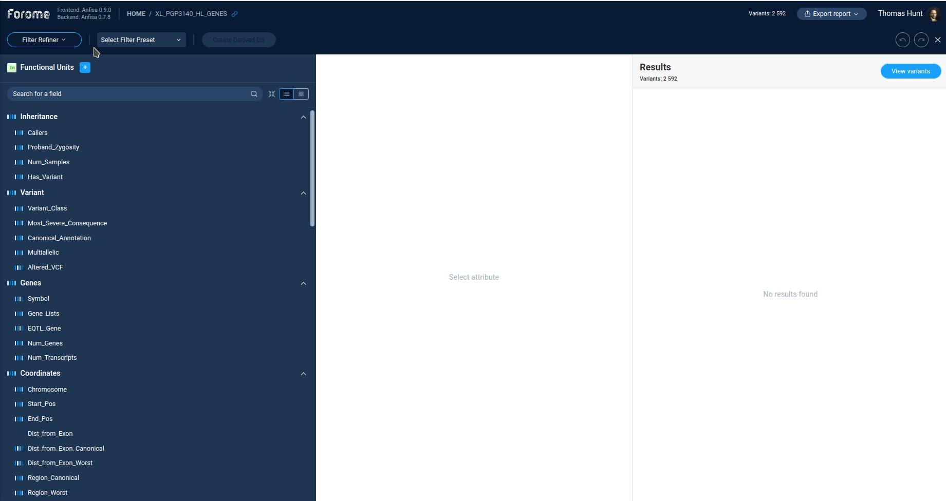
Main Filter refiner window
The caption of the Filter Refiner window contains the set of controls. The left one displays the work mode: Filter Refiner. Next to it user can select and create filter presets. Finally, the user can create a derived dataset for filtered ones.
Filters
Below the caption string, there is a list of available filters.
The Anfisa provides the user the large set of available filters for almost all variation properties in the initial VCF file. By clicking on each filter user can see the filter settings and details.
Full list of available filters with descriptions are available here: Filtering functions
By operation mode, all filters can be divided into two groups:
Categorical
Numeric
Categorical filters
Categorical data entries are presented by a list of filtering categories. On the filter details page, AnFiSA shows histogram or pie chart of categories distribution. User can select/deselect categories from the list.
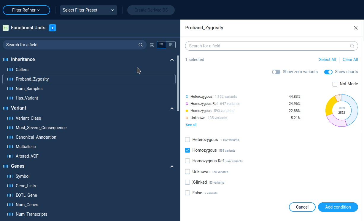
Only variants from selected categories will go to subsequent analysis. The Not Mode inverts the variations selection.
Numeric filters
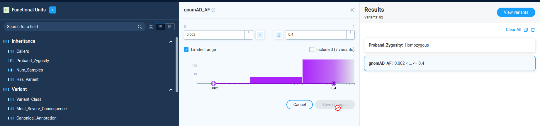
The numeric filters allows user to filter variations by the value of some numerical parameter. On the filter details page, AnFiSA shows histogram of value distribution. The distribution histogram is displayed in linear or logarithmic scale. The display mode is pre-configured for the filter and can’t be changed by user.
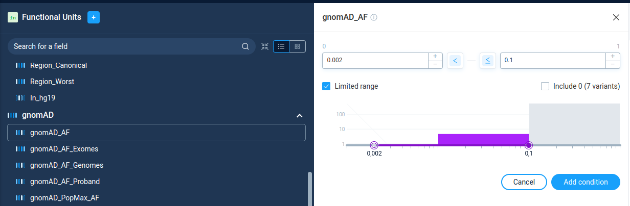
User can select value range either visually on the histogram or by typing the numeric values, or by clicking on the histogram. The buttons “<” and “<=” next to data entry edits controls incluson/exclusion of the border values.
The checkbox “Limited range” next to range selection forces user to choose parameter boundaries only inside the real parameter range for the current data set. This option is selected by default. For individual dataset analysis there is no sense in unchecking this option. However, for building preset to process different data sets, user can unselect this checkbox and have more flexibility in region selection.
Each numeric filter passes variations with the parameter value inside the specified range. In Filter Refiner mode there is no way to select variations outside the selected range. To do this, one can use the Decision tree functionality.
Filter discriminative power
In the context of Anfisa application there is a wide list of variant properties that can be used to reduce the number of selected variants. The Discriminative Power value is a special number used to help the user to notice the most “effective” properties from a long list.
Here “Effectivity” of a filter means that with use of it one can split the current set of variants on the most strongly differing groups (e.g. with loss maximum of “entropy”). So, the Discriminative Power in this context pure informational effectiveness, with no concerns of property meanings. The “effective” filter can separate variations into most differing groups, but this differentiation can have no real biological meaning.
The algorithm of discriminative power calculation is described here: Discriminative Power specification
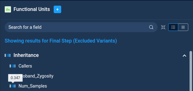
The visualization of this “effectivity” is an indicator with a choice of 3 or 4 colors close to the name of each filter. Each interval of discriminative power value has its own color coding, representing the number of different groups and number of variations in each group. This is a rough tool, however it might be helpful in work with a wide list of variants and filters.
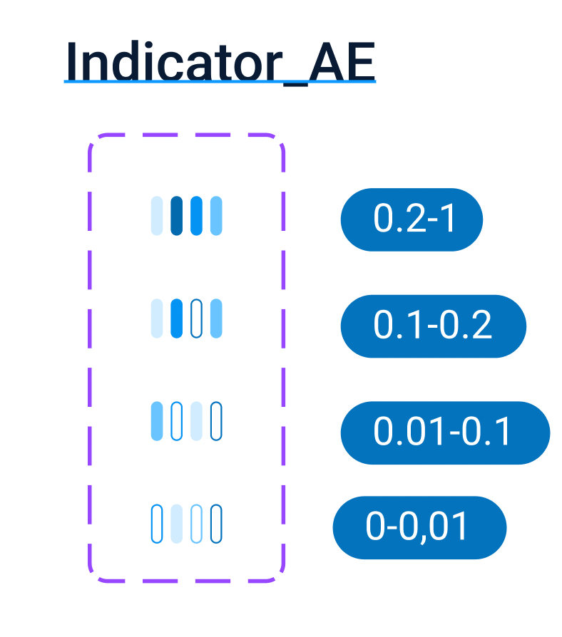
To see the exact value of discriminative power one can hover a mouse over the filter discriminative power indicator.
Filter chain creation
After setting filtering options for the filter, user applies it by pressing the Add condition button on th filter details page. After pressing this button, the new filter will be added to the list of filters on the right panel Results.
User can continue filtering process by adding new filters to the list. Anfisa allows to apply to a dataset combinations of filters and each additional filter operates on the result output of the previous filtering. The consequent application of different filters results only in conjunctions of the conditions.
On the Results panel, user can see all active filters, view and change filter settings. After filter settings change user need to press Save changes button to apply it. User can continue refinement process and add new filter to narrow the variations set.
Also AnFiSA displays the number of variants passing filter chain next to the panel caption: “Variants: 837”
User can delete an active filter by selecting pit and pressing the “Garbage bin” icon on the right of the Results panel. Or user can delete all filters by pressing the Clear All button.
Filtering chain functioning notes
Each new filter is applied to the already filtered variations set. Therefore adding each new filter will lead to narrowing of the variation set. To achieve more flexible filtering one should use Decision tree capability.
All charts in the filter details panel also displays the statistics for variations filtered by previous filters, not for original variations set.
Functional Units (Filtering functions)
The Functional units (filtering functions) are specific types of filtering actions.
From the user point of view they are very similar to “ordinary” filters. The difference is that “ordinary” filters use only data fields already present in the dataset. They utilise standard functionality of OLAP database and works very fast even on large sets of data. Also, all “regular” filters are commutative: they can be applied in any order and will produce the same result. This is the requirement of OLAP data analysis platform.
Filtering functions perform some calculations to filter data which has to be done interactively and can’t be precalculated in advance. They are not commutative and recommended to appy only after narrowing down the dataset size by “ordinary” filters
Functional units are accessible via specific popup on top of the filter list. For now AnFiSA implements only five functions.
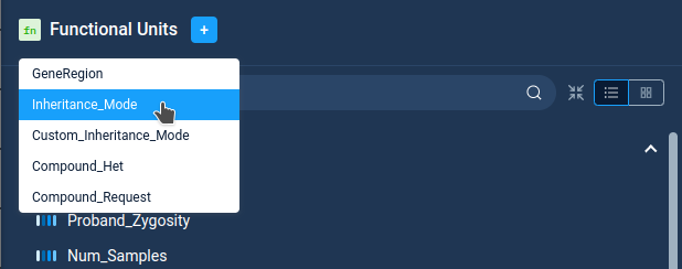
Functional units requires proper settings to work, which can be complicated in case of complex functions. Most part of currently implemented functions are associated with zygosity calculations and described in the separate section Notes on Zygosity.
Full description of functional units with required parameters is here: Filtering functions The description of filtering functions scientific applications can be found in AnFiSA paper
Data size for filtering functions
Most part of complex filtering functions (for example Compound_Request()) produce proper result only for valuable size of input data set. If input data contain to much variations the filtering results will not have any sense from the scientific point of view. In this case, AnFiSA stops calculation and returns an error message. This prevents user from making methodological errors in formally correct analysis.
The error message regarding too large data size is not just a technical limitation. In most cases, it means that your results does not have a sense from scientific point of view.
The same logic works for several other types of analysis and filtering, and even for the visual representation of the data.
Presets
User can save a created set of filters by pressing the Create preset button. User should provide the preset name and optionally assign a solution pack – the group of presets. To load a preset, user just needs to select a preset in a combo-box on the Filter Refiner caption.
The list of all available filter presets can be found here: Predefined filters
Viewing and saving filtration result
At the each step of data processing, user can view the filtering results by pressing the View variants button next to Results panel caption. AnFiSA displays the variations table in a new modal window. The button is active only if there are not more than 10000 variations in results.
The variation view window is in fact a limited version of the variation view table, available for secondary datasets. It is designed to be lightweight and fast, therefore it has only a limited set of functions.
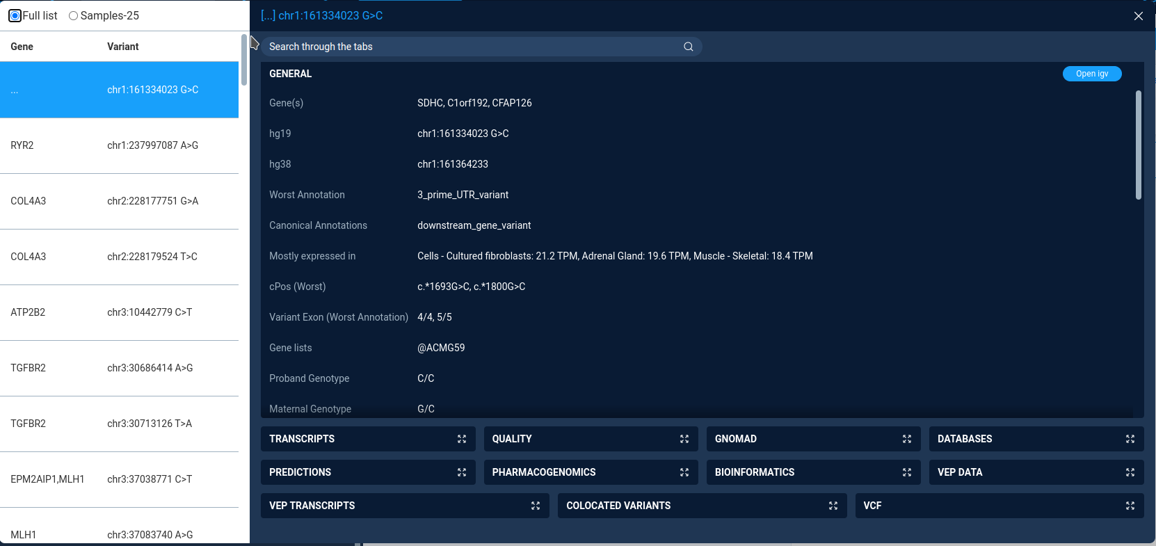
The left part of the window contains table with all variations and genes, affected by the variation.
The combobox on top of the variations table defines the variations view mode:
Samples-25 - display 25 randomly selected variations. Selected by default
Full list - display all variations. Available only is filtered set contains less than 300 variations.
The right part of the window displays the detailed data for selected variations. The variation properties are grouped by type in the collapsed boxes. User can expand any box by clicking on it.
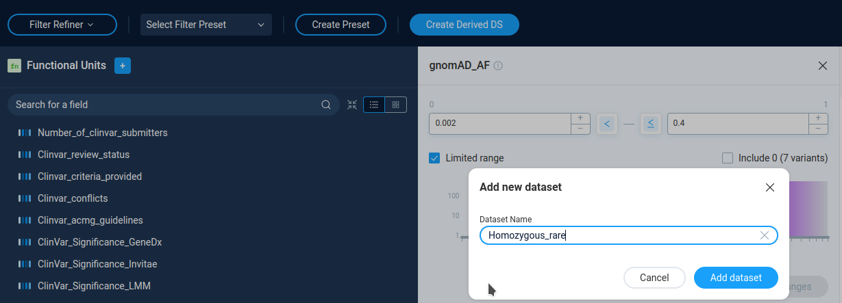
Creating a derived data set
User can save the resulting set of the variations as a derived dataset by pressing the Create Derived DS button and providing dataset name. The derived datasets are described in the corresponding section of the manual.
After creating a derived dataset user can either open derived dataset, or continue refining data.
Next: Decision Tree